Government#
In OG-Core, the government enters by levying taxes on households, providing transfers to households, levying taxes on firms, spending resources on public goods and infrastructure, and making rule-based adjustments to stabilize the economy in the long-run. It is this last activity that is the focus of this chapter.
Government Tax and Transfer Policy#
Government levies taxes on households and firms, funds public pensions, and makes other transfers to households.
Taxes#
Individual income taxes#
Income taxes are modeled through the net tax liability function for each household \(tax_{j,s,t}\), which can be decomposed into the effective tax rates times total income and wealth, respectively, (57). In this chapter, we detail the household tax component of government activity \(tax_{j,s,t}\) in OG-Core, along with our method of incorporating detailed microsimulation data into a dynamic general equilibrium model.
Incorporating realistic tax and incentive detail into a general equilibrium model is notoriously difficult for two reasons. First, it is impossible in a dynamic general equilibrium model to capture all of the dimensions of heterogeneity on which the real-world tax rate depends. For example, a household’s tax liability in reality depends on filing status, number of dependents, many types of income, and some characteristics correlated with age. A good heterogeneous agent DGE model tries to capture the most important dimensions of heterogeneity, and necessarily neglects the other dimensions.
The second difficulty in modeling realistic tax and incentive detail is the need for good microeconomic data on the individuals who make up the economy from which to simulate behavioral responses and corresponding tax liabilities and tax rates.
OG-Core follows the method of [DeBacker et al., 2019] of generating detailed tax data on effective tax rates and marginal tax rates for a sample of tax filers along with their respective income and demographic characteristics and then using that data to estimate parametric tax functions that can be incorporated into OG-Core.
Effective and Marginal Tax Rates#
Before going into more detail regarding how we handle these two difficulties in OG-Core, we need to define some functions and make some notation. For notational simplicity, we will use the variable \(x\) to summarize labor income, and we will use the variable \(y\) to summarize capital income.
We can express household net tax liability \(tax_{j,s,t}\) from the household budget constraint (22) as an effective tax rate on income multiplied by total income plus an effective tax rate on wealth multiplied by wealth \(b_{j,s,t}\),
where the wealth tax function is described in Section Wealth taxes of this chapter. Rearranging the first term on the right-hand-side of (57) gives the definition of an effective tax rate on income (\(\tau_{s,t}^{etr,xy}\)) as total tax liability, minus the wealth tax liability, divided by unadjusted gross income. And the definition of the effective tax rate on wealth (\(\tau_{t}^{etr,w}\)) as total tax liability, minus the income tax liability, divided by wealth.
A marginal tax rate (\(\tau_{s,t}^{mtr}\)) is defined as the change in total tax liability from a small change in either income or wealth. We allow these functions to vary by age \(s\) and time \(t\). In OG-Core, we differentiate between the marginal tax rate on labor income (\(\tau_{s,t}^{mtrx}\)), the marginal tax rate on capital income (\(\tau_{s,t}^{mtry}\)), and the marginal tax rate on wealth (\(\tau_{t}^{mtrw}\)).
Note that a change in wealth \(b_{j,s,t}\) changes both income tax liability (through capital income) and wealth tax liability. However, it is both intuitively and computationally convenient to defined the marginal tax rate on capital income and the marginal tax rate on wealth to be separate, as we have done here.
As we show in Section Optimality Conditions of the Households chapter of the OG-Core repository documentation, the derivative of total tax liability with respect to labor supply \(\frac{\partial tax_{j,s,t}}{n_{j,s,t}}\) and the derivative of total tax liability next period with respect to savings \(\frac{\partial tax_{j,s+1,t+1}}{b_{j,s+1,t+1}}\) show up in the household Euler equations for labor supply and savings , respectively, in the OG-Core documentation. It is valuable to be able to express those marginal tax rates, for which we have no data, as marginal tax rates for which we do have data. The following two expressions show how the marginal tax rates of labor supply can be expressed as the marginal tax rate on labor income times the household-specific wage and how the marginal tax rate of savings can be expressed as the marginal tax rate of capital income times the interest rate.
Fitting Tax Functions#
In looking at the 2D scatter plot on effective tax rates as a function of total income in Figure 2 and the 3D scatter plots of \(ETR\), \(MTRx\), and \(MTRy\) in Figure 3, it is clear that all of these rates exhibit negative exponential or logistic shape. This empirical regularity allows us to make an important and nonrestrictive assumption. We can fit parametric tax rate functions to these data that are constrained to be monotonically increasing in labor income and capital income. This assumption of monotonicity is computationally important as it preserves a convex budget set for each household, which is important for being able to solve many household lifetime problems over a large number of periods.
Default Tax Functional Form#
For the default option, OG-Core follows the approach of [DeBacker et al., 2019] in using the following functional form to estimate tax functions for each age \(s=E+1, E+2, ... E+S\) in each time period \(t\). This option can be manually selected by setting the parameter tax_func_type="DEP". Alternative specifications are outlined in Section Alternative Functional Forms below. Equation (63) is written as a generic tax rate, but we use this same functional form for \(ETR\)’s, \(MTRx\)’s, and \(MTRy\)’s.
The parameters values will, in general, differ across the different functions (effective and marginal rate functions) and by age, \(s\), and tax year, \(t\). We drop the subscripts for age and year from the above exposition for clarity.
By assuming each tax function takes the same form, we are breaking the analytical link between the the effective tax rate function and the marginal rate functions. In particular, one could assume an effective tax rate function and then use the analytical derivative of that to find the marginal tax rate function. However, we’ve found it useful to separately estimate the marginal and average rate functions. One reason is that we want the tax functions to be able to capture policy changes that have differential effects on marginal and average rates. For example, a change in the standard deduction for tax payers would have a direct effect on their average tax rates. But it will have secondary effect on marginal rates as well, as some filers will find themselves in different tax brackets after the policy change. These are smaller and second order effects. When tax functions are are fit to the new policy, in this case a lower standard deduction, we want them to be able to represent this differential impact on the marginal and average tax rates. The second reason is related to the first. As the additional flexibility allows us to model specific aspects of tax policy more closely, it also allows us to better fit the parameterized tax functions to the data.
The key building blocks of the functional form Equation (63) are the \(\tau(x)\) and \(\tau(y)\) univariate functions. The ratio of polynomials in the \(\tau(x)\) function \(\frac{Ax^2 + Bx}{Ax^2 + Bx + 1}\) with positive coefficients \(A,B>0\) and positive support for labor income \(x>0\) creates a negative-exponential-shaped function that is bounded between 0 and 1, and the curvature is governed by the ratio of quadratic polynomials. The multiplicative scalar term \((max_x-min_x)\) on the ratio of polynomials and the addition of \(min_x\) at the end of \(\tau(x)\) expands the range of the univariate negative-exponential-shaped function to \(\tau(x)\in[min_x, max_x]\). The \(\tau(y)\) function is an analogous univariate negative-exponential-shaped function in capital income \(y\), such that \(\tau(y)\in[min_y,max_y]\).
The respective \(shift_x\) and \(shift_y\) parameters in Equation (63) are analogous to the additive constants in a Stone-Geary utility function. These constants ensure that the two sums \(\tau(x) + shift_x\) and \(\tau(y) + shift_y\) are both strictly positive. They allow for negative tax rates in the \(\tau(\cdot)\) functions despite the requirement that the arguments inside the brackets be strictly positive. The general \(shift\) parameter outside of the Cobb-Douglas brackets can then shift the tax rate function so that it can accommodate negative tax rates. The Cobb-Douglas share parameter \(\phi\in[0,1]\) controls the shape of the function between the two univariate functions \(\tau(x)\) and \(\tau(y)\).
This functional form for tax rates delivers flexible parametric functions that can fit the tax rate data shown in the scatterplot data in Figure 2 and Figure 3 as well as a wide variety of policy reforms. Further, these functional forms are monotonically increasing in both labor income \(x\) and capital income \(y\). This characteristic of monotonicity in \(x\) and \(y\) is essential for guaranteeing convex budget sets and thus uniqueness of solutions to the household Euler equations. The assumption of monotonicity does not appear to be a strong one when viewing the the tax rate data shown in Figure 3. While it does limit the potential tax systems to which one could apply our methodology, tax policies that do not satisfy this assumption would result in non-convex budget sets and thus require non-standard DGE model solutions methods and would not guarantee a unique equilibrium. The 12 parameters of our tax rate functional form from (63) are summarized in Table 1.
Symbol |
Description |
|---|---|
\(A\) |
Coefficient on squared labor income term \(x^2\) in \(\tau(x)\) |
\(B\) |
Coefficient on labor income term \(x\) in \(\tau(x)\) |
\(C\) |
Coefficient on squared capital income term \(y^2\) in \(\tau(y)\) |
\(D\) |
Coefficient on capital income term y in \(\tau(y)\) |
\(max_{x}\) |
Maximum tax rate on labor income \(x\) given \(y\) = 0 |
\(min_{x}\) |
Minimum tax rate on labor income \(x\) given \(y\) = 0 |
\(max_{y}\) |
Maximum tax rate on capital income \(y\) given \(x\) = 0 |
\(min_{y}\) |
Minimum tax rate on capital income \(y\) given \(x\) = 0 |
\(shift_{x}\) |
shifter \(> \|min_{x}\|\) ensures that \(\tau(x,y)\) + \(shift_{x} \geq 0\) despite potentially negative values for \(\tau(x)\) |
\(shift_{y}\) |
shifter \(> \|min_{y}\|\) ensures that \(\tau(x,y)\) + \(shift_{y} \geq 0\) despite potentially negative values for \(\tau(y)\) |
\(shift\) |
shifter (can be negative) allows for support of \(\tau(x,y)\) to include negative tax rates |
\(\phi\) |
Cobb-Douglas share parameter between 0 and 1 |
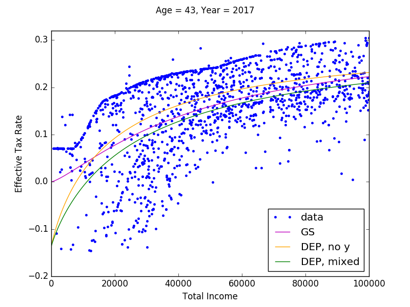
Fig. 2 Plot of estimated \(ETR\) functions: \(t=2017\) and \(s=43\) under current law#
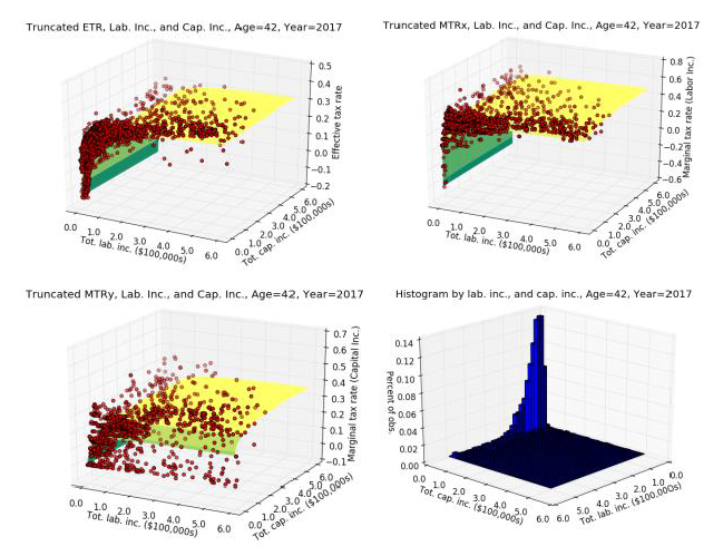
Fig. 3 Estimated tax rate functions of ETR, MTRx, MTRy, and histogram as functions of labor income and capital income from microsimulation model: \(t=2017\) and \(s=42\) under 2017 law in the United States. Note: Axes in the histogram in the lower-right panel have been switched relative to the other three figures in order to see the distribution.#
Parameter |
\(ETR\) |
\(MTRx\) |
\(MTRy\) |
|---|---|---|---|
\(A\) |
6.28E-12 |
3.43E-23 |
4.32E-11 |
\(B\) |
4.36E-05 |
4.50E-04 |
5.52E-05 |
\(C\) |
1.04E-23 |
9.81E-12 |
5.62E-12 |
\(D\) |
7.77E-09 |
5.30E-08 |
3.09E-06 |
\(max_{x}\) |
0.80 |
0.71 |
0.44 |
\(min_{x}\) |
-0.14 |
-0.17 |
0.00E+00 |
\(max_{y}\) |
0.80 |
0.80 |
0.13 |
\(min_{y}\) |
-0.15 |
-0.42 |
0.00E+00 |
\(shift_{x}\) |
0.15 |
0.18 |
4.45E-03 |
\(shift_{y}\) |
0.16 |
0.43 |
1.34E-03 |
\(shift\) |
-0.15 |
-0.42 |
0.00E+00 |
\(\phi\) |
0.84 |
0.96 |
0.86 |
Obs. (\(N\)) |
3,105 |
3,105 |
1,990 |
SSE |
9,122.68 |
15,041.35 |
7,756.54 |
Let \(\boldsymbol{\theta}_{s,t}=(A,B,C,D,max_x,min_x,max_y,min_y,shift_x,shift_y,shift,\phi)\) be the full vector of 12 parameters of the tax function for a particular type of tax rate, age of filers, and year. We first directly specify \(min_x\) as the minimum tax rate and \(max_x\) as the maximum tax rate in the data for age-\(s\) and period-\(t\) individuals for capital income close to 0 (\(\$0<y<\$3,000\)), and \(min_y\) as the minimum tax rate and \(max_y\) as the maximum tax rate for labor income close to 0 (\(\$0<x<\$3,000\)). We then set \(shift_x = \min(0,|min_x|)+\epsilon\) and \(shift_y = \min(0,|min_y|)+\epsilon\) so that the respective arguments in the brackets of (63) are strictly positive. Then let \(shift\) be be the minimum tax rate in the corresponding data minus \(\epsilon\). Let \(\bar{\boldsymbol{\theta}}_{s,t}=\{min_x,max_x,min_y,max_y,shift_x,shift_y, shift\}\) be the set of parameters we take directly from the data in this way.
We then estimate five remaining parameters \(\tilde{\boldsymbol{\theta}}_{s,t}=(A,B,C,D,\phi)\) using the following nonlinear weighted least squares criterion,
where \(\tau_{i}\) is the tax rate for observation \(i\) from the microsimulation output, \(\tau_{s,t}(x_i,y_i|\tilde{\boldsymbol{\theta}}_{s,t},\bar{\boldsymbol{\theta}}_{s,t})\) is the predicted tax rate for filing-unit \(i\) with \(x_{i}\) labor income and \(y_{i}\) capital income given parameters \(\boldsymbol{\theta}_{s,t}\), and \(w_{i}\) is the CPS sampling weight of this observation. The number \(N\) is the total number of observations from the microsimulation output for age \(s\) and year \(t\). Figure 3 shows the typical fit of an estimated tax function \(\tau_{s,t}\bigl(x,y|\hat{\boldsymbol{\theta}}_{s,t}\bigr)\) to the data for \(s=42\) and year \(t=2017\).
The underlying data can limit the number of tax functions that can be estimated. For example, we use the age of the primary filer from the PUF-CPS match to be equivalent to the age of the DGE model household. The DGE model we use allows for individuals up to age 100, however the data contain few primary filers with age above age 80. Because we cannot reliably estimate tax functions for \(s>80\), we apply the tax function estimates for 80 year-olds to those with model ages 81 to 100. In the case certain ages below age 80 have too few observations to enable precise estimation of the model parameters, we use a linear interpolation method to find the values for those ages \(21\leq s <80\) that cannot be precisely estimated. [1]
In OG-Core, we estimate the 12-parameter functional form (63) using weighted nonlinear least squares to fit an effective tax rate function \((\tau^{etr}_{s,t})\), a marginal tax rate of labor income function \((\tau^{mtrx}_{s,t})\), and a marginal tax rate of capital income function \((\tau^{mtry}_{s,t})\) for each age \(E+1\leq s\leq E+S\) and each of the first 10 years from the current period. [2] That means we have to perform 2,400 estimations of 12 parameters each. Figure 3 shows the predicted surfaces for \(\tau^{etr}_{s=42,t=2017}\), \(\tau^{mtrx}_{s=42,t=2017}\), and \(\tau^{mtry}_{s=42,t=2017}\) along with the underlying scatter plot data from which those functions were estimated. Table 2 shows the estimated values of those functional forms.
Alternative Functional Forms#
In addition to the default option using tax functions of the form developed by [DeBacker et al., 2019], OG-Core also allows users to specify alternative tax functions. Four alternatives are offered:
Functions as in [DeBacker et al., 2019], but where \(\tau^{etr}_{s,t}\), \(\tau^{mtrx}_{s,t}\), and \(\tau^{mtry}_{s,t}\) are functions of total income (i.e., \(x+y\)) and not labor and capital income separately. Users can select this option by setting the parameter
tax_func_type="DEP_totalinc".Functions of the Gouveia and Strauss form [Gouveia and Strauss, 1994]:
\[ \tau = \phi_{0}(1 - (x+y)^{(\phi_{1}-1)}((x+y)^{-\phi_{1}} + \phi_{2})^{(-1 - \phi_{1})/\phi_{1}})\]Users can select this option by setting the parameter
tax_func_type="GS". The three parameters of this function (\(\phi_{0}, \phi_{1}, \phi_{2}\)) are estimated using the weighted sum of squares estimated described in Equation (64).Tax functions from [Heathcote et al., 2017]:
\[ \tau = 1 - \phi_{0}(x+y)^{1-phi_1}\]Users can select this option by setting the parameter
tax_func_type="HSV". The two parameters of this function (\(\phi_{0}, \phi_{1}\)) are estimated using ordinary least squares.Linear tax functions (i.e., \(\tau =\) a constant). Users can select this option by setting the parameter
tax_func_type="linear". The constant rate is found by taking the weighted average of the appropriate tax rate (effective tax rate, marginal tax rate on labor income, marginal tax rate on labor income) for each age and year, where the values are weighted by sampling weights and income.Monotonically increasing smoothing spline
tax_func_type="mono". This functional approach is based on [Eilers and Marx, 1996], [Eilers, 2003] and [Eilers, 2005], which is a least squares smoothing spline that penalizes nonmonotonicities. We used k-fold cross validation to show that the optimal smoothing parameter for this function on our tax data is \(\lambda=12\), which is set as the default. These tax functions are fit to total income data (labor income plus capital income).
Among all of these tax functional forms, users can set the age_specific parameter to False if they wish to have one function for all ages \(s\). In addition, for the functions based on [DeBacker et al., 2019] (tax_func_type="DEP" or tax_func_type="DEP_totinc"), one can set analytical_mtrs=True if they wish to have the \(\tau^{mtrx}_{s,t}\) and \(\tau^{mtry}_{s,t}\) derived from the \(\tau^{etr}_{s,t}\) functions. This provides theoretical consistency, but reduced fit of the functions (see [DeBacker et al., 2019] for more details).
Income Tax Noncompliance#
The parameters of the tax functions used in OG-Core are typically estimated using data that miss the effects of compliance (either because they use administrative data from tax returns or because of similar under-reporting in survey data [Hurst et al., 2014](see Hurst et al. (REStat, 2014))). OG-Core therefore offers the user two parameters that scale the marginal and effective tax rate functions in order to account for income tax noncompliance. These parameters are labor_income_tax_noncompliance_rate and capital_income_tax_noncompliance_rate and represent the rates of noncompliance on the respective sources of income. The implementation of these parameters is as follows. Let represent \(\eta\) the noncompliance rate (on labor and capital income) and let \(\tau\) represent the marginal tax rate (on labor or capital income) without accounting for noncompliance. Then, the marginal tax rate faced by a household, after accounting for compliance decisions, is \(\tau^{nc} = (1 - \eta)\tau\).
When computing the role of compliance on the effective tax rate, we take a weighted average over the rates of noncompliance for labor and capital income. If we let \(X\) represent labor income, \(Y\) capital income, and \(\eta_X\) and \(\eta_Y\) represent the noncompliance rates on labor and capital income, respecitvely. Then the noncompliance rate applied to the effective tax rate is given by \(\eta = \frac{\eta_X X + \eta_Y Y}{X + Y}\). If we use \(\tau\) to represent the effective tax rate, then the effective tax rate used in the households budget constraint and to determine tax liability is \(\tau^{nc} = (1 - \eta)\tau\), where the \(\eta\) represents the average rate of noncompliance across income sources.
Factor Transforming Income Units#
The tax functions \(\tau^{etr}_{s,t}\), \(\tau^{mtrx}_{s,t}\), and \(\tau^{mtry}_{s,t}\) are typcically estimated on data with income in current currency units. However, the consumption units of the OG-Core model are not in the same units as the real-world income data. For this reason, we have to transform the income by a \(factor\) so that it is in the same units as the income data on which the tax functions were estimated.
The tax rate functions are each functions of capital income and labor income \(\tau(x,y)\). In order to make the tax functions return accurate tax rates associated with the correct levels of income, we multiply the model income \(x^m\) and \(y^m\) by a \(factor\) so that they are in the same units as the real-world U.S. income data \(\tau(factor\times x^m, factor\times y^m)\). We define the \(factor\) such that average steady-state household total income in the model times the \(factor\) equals the U.S. data average total income.
We do not know the steady-state wage, interest rate, household labor supply, and savings ex ante. So the income \(factor\) is an endogenous variable in the steady-state equilibrium computational solution. We hold the factor constant throughout the nonsteady-state equilibrium solution.
Consumption taxes#
Linear consumption taxes, \(\tau^c_{i,t}\) can vary over time and by consumption good.
Wealth taxes#
Wealth taxes can be implemented through the \(tax^{w}_{j,s,t}(b_{j,s,t})\) function, shown in equations (57) through (62). This functional form allows for zero to flat to progressive wealth taxation and is given by the following,
where \(p^w\geq 0\) is a nonnegative scale parameter of the overall tax rate, \(h^w> 0\) is a strictly positive scale coefficient parameter on the linear term inside of the parentheses, and \(m^w\geq 0\) is a nonnegative constant additive coefficient in the denominator of the rate function in parentheses. This functional form allows us to represent a zero wealth tax rate (\(p^w=0\)), a flat wealth tax rate (\(p^w>0\) and \(m_w= 0\)), and a progressive wealth tax rate (\(p^w\), \(h^w\), and \(m^w\) > 0).
The expression for the effective tax rate on wealth is the following.
The analytical expression for the marginal tax rate on wealth defined in equation {eq}`` is the following.
Corporate income taxes#
Businesses face a linear tax rate \(\tau^{corp}_{m,t}\), which can vary by industry and over time. In the case of a single industry, OG-Core provides the parameters c_corp_share_of_assets to scale the tax rate applied to the representative firm so that it represents a weighted average between the rate on businesses entities taxes at the entity level (e.g., C corporations in the United States) and those with no entity level tax. The parameter adjustment_factor_for_cit_receipts is additionally provided to represent a wedge between marginal and average tax rates (which could otherwise be zero with a linear tax function).
Spending#
Government spending is comprised of government provided pension benefits, lump sum transfers, universal basic income payments, infrastructure investment, spending on public goods, and interest payments on debt. Below, we describe the transfer spending amounts. Spending on infrastructure, public goods, and interest are described in Government Budget Constraint. Because government spending on lump-sum transfers to households \(TR_t\), public goods \(G_t\), and government infrastructure capital \(I_g\) are all functions of nominal GDP, we define GDP here,
where GDP \(Y_t\) is in terms of the numeraire good of industry-\(M\) output.[3]
Pensions#
The OG-Core model allows for four different systems for public pensions:
U.S.-style social security system
Defined benefit system
Notional defined contribution system
Points system
These can be selected with the pension_system parameter. Accepted values are US-Style Social Security, Defined Benefits, Notional Defined Contribution, Points System. We discuss each of these in turn below.
For all systems, \(R\) represents the age at which the individual becomes eligible to receive the government provided retirement benefit.
Defined benefit system#
The defined benefit system pension amount is given as:
where:
\(ny\) are the number of years over which average earnings are calculated
\(Cy\) are the number of years of contributions. In our model, there is no exit from the labor force, so workers will contribute for \(R\) years, but \(Cy\) could be some number less than \(R\) if there is a maximum number of years of contributions one can accrue under the DB system.
\(\alpha_{DB}\) is the replacement rate per year of contribution.
Given this pension system and the fact that there is only variation in labor supply along the intensive margin (so we don’t need to consider changes in \(Cy\)), the partial derivatives from the household section are given by:
Notional defined contribution system#
The pension amount under a notional defined contribution system is given as:
where:
\(\tau^p\) is the pension contribution tax rate
\(g_{NDC,t}\) the rate of growth applied to contributions.
For example, In the Italian system, \(g_{NDC,t}\) is the mean nominal GDP growth rate in the 5 years before seniority
i.e., \(g_{NDC,t}=\prod_{j=i}^{R-1}\bar{g}_{j}\)
Note, this is not \(g_y\). In the SS, it’s \((\bar{g}_{y} + \bar{g}_{n})\), and in the transition path equilibrium, it’s not a function of exogenous variables since the growth rate of nominal GDP is endogenous.
\(\delta_{R, t}\) is the conversion coefficient at time \(t\) and its calculation is detailed below.
where \(k\) is an adjustment that takes into account the number of payments per year. In particular, \(k=0.5 - (6/13n)\), where \(n\) is the number of payments per year. So if the payments are made monthly, \(n=12\) and thus \(k=0.4615\).
The \(dir_{R, t}\) term is an adjustment to make the payments actuarially fair given mortality risk:
where \(\hat{\rho}_{s,t}\) are the mortality tables used in the pension system at time \(t\) and \(\hat{g}_{y, t}\) is the long run expected nominal GDP growth rate used in the pension system at time \(t\).
Finally, \(ind_{R}\) is an adjustment for survivor benefits. Since we model households (and not individuals), we set \(ind_{R} = 0\) by default. This can be changed with the parameter indR if one would like to account for the fact that households lose members over time.
Given this pension system, the partial derivatives from the household section are given by:
Points system#
Under a points system, the pension amount is given as:
where \(v_{t}\) is the value of a point at time \(t\)
Given this pension system, the partial derivatives from the household section are given by:
Aggregate Pension Spending#
Total pension spending is the sum of the pension payments to each household in the model:
Lump sum transfers:#
Aggregate non-pension transfers to households are assumed to be a fixed fraction \(\alpha_{tr}\) of GDP each period:
The time dependent multiplier \(g_{tr,t}\) in front of the right-hand-side of (81) will equal 1 in most initial periods. It will potentially deviate from 1 in some future periods in order to provide a closure rule that ensures a stable long-run debt-to-GDP ratio. We will discuss the closure rule in Section Budget Closure Rule.
Universal basic income#
[TODO: This section is far along but needs to be updated.]
Universal basic income (UBI) transfers show up in the household budget constraint (22). Household amounts of UBI can vary by household age \(s\), lifetime income group \(j\), and time period \(t\). These transfers are represented by \(ubi_{j,s,t}\).
Calculating UBI#
Household transfers in model units of the numeraire good \(ubi_{j,s,t}\) are a function of five policy parameters described in the default_parameters.json file (ubi_growthadj, ubi_nom_017, ubi_nom_1864, ubi_nom_65p, and ubi_nom_max). Three additional parameters provide information on household structure by age, lifetime income group, and year: [ubi_num_017_mat, ubi_num_1864_mat, ubi_num_65p_mat].
As a convenience to users, UBI policy parameters ubi_nom_017, ubi_nom_1864, ubi_nom_65p, and ubi_nom_max are entered as nominal amounts (e.g., in dollars or pounds). The parameter ubi_nom_017 represents the nominal value of the UBI transfer to each household per dependent child age 17 and under. The parameter ubi_nom_1864 represents the nominal value of the UBI transfer to each household per adult between the ages of 18 and 64. And ubi_nom_65p is the nominal value of UBI transfer to each household per senior 65 and over. The maximum UBI benefit per household, ubi_nom_max, is also a nominal amount. From these parameters, the model computes nominal UBI payments to each household in the model:
The rest of the time periods of the household UBI transfer and the respective steady-states are determined by whether the UBI is growth adjusted or not as given in the ubi_growthadj boolean parameter. The following two sections cover these two cases.
UBI specification not adjusted for economic growth#
A non-growth adjusted UBI (ubi_growthadj = False) is one in which the initial nonstationary nominal-valued \(t=0\) UBI matrix \(ubi^{nom}_{j,s,t=0}\) does not grow, while the economy’s long-run growth rate is \(g_y\) for the most common parameterization is positive (\(g_y>0\)).
As described in chapter Stationarization, the stationarized UBI transfer to each household \(\hat{ubi}_{j,s,t}\) is the nonstationary transfer divided by the growth rate since the initial period. When the long-run economic growth rate is positive \(g_y>0\) and the UBI specification is not growth-adjusted, the steady-state stationary UBI household transfer is zero \(\overline{ubi}_{j,s}=0\) for all lifetime income groups \(j\) and ages \(s\) as time periods \(t\) go to infinity. However, to simplify, we assume in this case that the stationarized steady-state UBI transfer matrix to households is the stationarized value of that matrix in period \(T\).[4]
Note that in non-growth-adjusted case, if \(g_y<0\), then the stationary value of \(\hat{ubi}_{j,s,t}\) is going to infinity as \(t\) goes to infinity. Therefore, a UBI specification must be growth adjusted for any assumed negative long run growth \(g_y<0\).[5]
UBI specification adjusted for economic growth#
Put description of growth-adjusted specification here.
Spending in the reform simulation#
While aggregate spending on \(G\), \(TR\), and \(I_g\) in the baseline simulation are set as fractions of GDP, in the reform simulation, these spending amounts can be set in two different ways. The method is controlled by the baseline_spending parameter. If baseline_spending=False, the behavior of these spending is analgous to that in the baseline simulation; they are set as fractions of GDP, in this case GDP in the reform simulation. Thus, with the default assumption of baseline_spending it’s assumed that spending levels in these three categories are function of GDP in the reform. In this case, users will see that, even with the parameters \(\alpha_G\), \(\alpha_T\), and \(\alpha_I\) are unchanged, the level of spending will change in the reform if GDP in the reform is different.
With the assumption of baseline_spending=True, the level of spending in the reform is held to the level of spending in the baseline. If the user wishes to adjust the level of spending, relative to the baseline level, in the reform, then the parameters alpha_bs_G, alpha_bs_T, and alpha_bs_I can be used to proportionally increase or decrease the levels of spending on \(G\), \(TR\), and \(I_g\) in the reform simulation, relative to the levels in the baseline simulation. Note that the alpha_bs_* parameters are time varying, so the proportional change in spending can be different across time. E.g., for government consumption expenditures, we’d have the reform amount of \(G\) determined as:
Note that the budget closure rule (described in Section ref{SecUnbalGBCcloseRule}) still takes effect in the case of baseline_spending=True. What this means is that the relation described above holds until the period in which the closure rules takes effect. Once the closure rule begins, the path of \(G\) (and/or \(TR\), depending on the closure rule used) will adjust as determined by the rule to close the government budget in the long run.
Government Tax Revenue#
We see from the household’s budget constraint that net taxes \(tax_{j,s,t}\) and government transfers \(tr_{j,s,t}\) enter into the household’s decision,
where we defined the tax liability function \(tax_{j,s,t}\) in (23) as effective tax rate times respective total income and wealth. The transfer distribution function \(\eta_{j,s,t}\) can vary by lifetime ability group \(j\), age \(s\), and time period \(t\). Households also remit tax on bequests received (\(\tau^{bq}\)) and on consumption (\(\tau^c\)). And government revenue from the corporate income tax rate schedule \(\tau^{corp}_{m,t}\) and the tax on depreciation expensing schedule \(\delta^\tau_{m,t}\) enters the firms’ profit function in each industry \(m\).
We define total government revenue from taxes in terms of the numeraire good as the following,
where household labor income is defined as \(x_{j,s,t}\equiv w_t e_{j,s}n_{j,s,t}\) and capital income \(y_{j,s,t}\equiv r_{p,t} b_{j,s,t}\).
Government Budget Constraint#
Let the level of government debt in period \(t\) be given by \(D_t\). The government budget constraint requires that government revenue \(Rev_t\), external foreign assistance, \(FA_t\), plus the budget deficit (\(D_{t+1} - D_t\)) equal expenditures on interest on the debt, government spending on public goods \(G_t\), total infrastructure investments \(I_{g,t}\), total pension outlays, total transfer payments to households \(TR_t\), and \(UBI_t\) every period \(t\),
where \(r_{gov,t}\) is the interest rate paid by the government defined in equation (94) below, \(G_{t}\) is government spending on public goods, \(I_{g,t}\) is total government spending on infrastructure investment, \(TR_{t}\) are non-pension government transfers, and \(UBI_t\) is the total UBI transfer outlays across households in time \(t\). All variables in (88) are real variables denominated in units of current-period output in industry \(M\) the numeraire (\(p_{M,t}=1\) for all \(t\)).
We assume that government spending on public goods in terms of the numeraire good is a fixed fraction of GDP each period in the initial periods.
Similar to transfers \(TR_t\), the time dependent multiplier \(g_{g,t}\) in front of the right-hand-side of (89) will equal 1 in most initial periods. It will potentially deviate from 1 in some future periods in order to provide a closure rule that ensures a stable long-run debt-to-GDP ratio. We make this more specific in the next section.
Total government infrastructure investment spending, \(I_{g,t}\) is assumed to be a time-dependent fraction of GDP.
The government also chooses what percent of total infrastructure investment goes to each industry \(\alpha_{I,m,t}\), although these are exogenously calibrated parameters in the model.
The stock of public capital (i.e., infrastructure) in each industry \(m\) evolves according to the law of motion,
where \(\delta_g\) is the depreciation rate on infrastructure and \(\phi_g\) (infra_investment_leakage_rate) is the fraction of infrastructure investment lost to leakage (e.g., corruption or other frictions). The stock of public capital in each industry \(m\) complements labor and private capital in the production function of the representative firm, in Equation (42).
Aggregate spending on UBI at time \(t\) is the sum of UBI payments across all households at time \(t\):
Interest Rate on Government Debt and Household Savings#
Despite the model having no aggregate risk, it may be helpful to build in an interest rate differential between the rate of return on private capital and the interest rate on government debt. Doing so helps to add realism by including a risk premium. OG-Core allows users to set an exogenous wedge between these two rates. OG-Core also allows for the risk premium on debt to be a quadratic function of the debt-to-GDP ratio. The interest rate on government debt is given by:
where \(r_t\) is the marginal product of capital faced by firms. The two parameters, \(\tau_{d,t}\) and \(\mu_{d,t}\) can be used to allow for a government interest rate that is a percentage hair cut from the market rate or a government interest rate with a constant risk premium. The parameters \(\beta_1\) and \(\beta_2\) can be used to allow for a quadratic risk premium on government debt that is a function of the debt-to-GDP ratio.
Budget Closure Rule#
If total government transfers to households \(TR_t\) and government spending on public goods \(G_t\) are both fixed fractions of GDP, one can imagine corporate and household tax structures that cause the debt level of the government to either tend toward infinity or to negative infinity, depending on whether too little revenue or too much revenue is raised, respectively.
A virtue of dynamic general equilibrium models is that the model must be stationary in the long-run in order to solve it. That is, no variables can be indefinitely growing as time moves forward. The labor augmenting productivity growth \(g_y\) from Chapter Firms and the potential population growth \(\tilde{g}_{n,t}\) from the calibration chapter on demographics in the country-specific repository documentation render the model nonstationary. But we show how to stationarize the model against those two sources of growth in Chapter Stationarization. However, even after stationarizing the effects of productivity and population growth, the model could be rendered nonstationary and, therefore, not solvable if government debt were becoming too positive or too negative too quickly.
For the model to be stationary, the debt-to-GDP ratio must be stable in the long run. Because the debt-to-GDP ratio is a quotient of two macroeconomic variables, the non-stationary and stationary versions of this ratio are equivalent. Let \(T\) be some time period in the future. The stationarizing assumption is the following,
where \(\alpha_D\) is a scalar long-run value of the debt-to-GDP ratio. This long-run stability condition on the debt-to-GDP ratio clearly applies to the steady-state as well as any point in the time path for \(t>T\).
We detail three possible closure-rule options here for stabilizing the debt-to-GDP ratio in the long run, although OG-Core only has the capability currently to execute the first closure rule that adjusts government spending \(G_t\). We expect to have the other two rules implemented as OG-Core options soon. Each rule uses some combination of changes in government spending on public goods \(G_t\) and government transfers to households \(TR_t\) to stabilize the debt-to-GDP ratio in the long-run.
Change only government spending on public goods \(G_t\).
Change only government transfers to households \(TR_t\).
Change both government spending \(G_t\) and transfers \(TR_t\) by the same percentage.
Change government spending only#
We specify a closure rule that is automatically implemented after some period \(T_{G1}\) to stabilize government debt as a percent of GDP (debt-to-GDP ratio) by period \(T_{G2}\). Let \(\alpha_D\) represent the long-run debt-to-GDP ratio at which we want the economy to eventually settle.
The first case in (96) says that government spending \(G_t\) will be a fixed fraction \(\alpha_g\) of GDP \(Y_t\) for every period before \(T_{G1}\). The second case specifies that, starting in period \(T_{G1}\) and continuing until before period \(T_{G2}\), government spending be adjusted to set tomorrow’s debt \(D_{t+1}\) to be a convex combination between its long-run stable level \(\alpha_D Y_t\) and the current debt level \(D_t\), where \(\alpha_D\) is a target debt-to-GDP ratio and \(\rho_d\in(0,1]\) is the percent of the way to jump toward the target \(\alpha_D Y_t\) from the current debt level \(D_t\). The last case specifies that, for every period after \(T_{G2}\), government spending \(G_t\) is set such that the next-period debt be a fixed target percentage \(\alpha_D\) of GDP.
Change government transfers only#
If government transfers to households are specified by (81) and the long-run debt-to-GDP ratio can only be stabilized by changing transfers, then the budget closure rule must be the following.
The first case in (97) says that government transfers \(TR_t\) will be a fixed fraction \(\alpha_{tr}\) of GDP \(Y_t\) for every period before \(T_{G1}\). The second case specifies that, starting in period \(T_{G1}\) and continuing until before period \(T_{G2}\), government transfers be adjusted to set tomorrow’s debt \(D_{t+1}\) to be a convex combination between the target debt \(\alpha_D Y_t\) and the current debt level \(D_t\). The last case specifies that, for every period after \(T_{G2}\), government transfers \(TR_t\) are set such that the next-period debt be a fixed target percentage \(\alpha_D\) of GDP.
Change both government spending and transfers#
In some cases, changing only government spending \(G_t\) or only government transfers \(TR_t\) will not be enough. That is, there exist policies for which a decrease in government spending to zero after period \(T_{G1}\) will not stabilize the debt-to-GDP ratio. And negative government spending on public goods does not make sense. [6] On the other hand, negative transfers do make sense. Notwithstanding, one might want the added stabilization ability of changing both government spending \(G_t\) and transfers \(TR_t\) to stabilize the long-run debt-to-GDP ratio.
In our specific form of this joint option, we assume that the factor by which we scale government spending and transfers is the same \(g_{g,t} = g_{tr,t}\) for all \(t\). We label this single scaling factor \(g_{trg,t}\).
If government spending on public goods is specified by (89) and government transfers to households are specified by (81) and the long-run debt-to-GDP ratio can only be stabilized by changing both spending and transfers, then the budget closure rule must be the following.
The first case in (99) says that government spending and government transfers \(TR_t\) will their respective fixed fractions \(\alpha_g\) and \(\alpha_{tr}\) of GDP \(Y_t\) for every period before \(T_{G1}\). The second case specifies that, starting in period \(T_{G1}\) and continuing until before period \(T_{G2}\), government spending and transfers be adjusted by the same rate to set tomorrow’s debt \(D_{t+1}\) to be a convex combination between target debt \(\alpha_D Y_t\) and the current debt level \(D_t\). The last case specifies that, for every period after \(T_{G2}\), government spending and transfers are set such that the next-period debt be a fixed target percentage \(\alpha_D\) of GDP.
Each of these budget closure rules (96), (97), and (99) allows the government to run increasing deficits or surpluses in the short run (before period \(T_{G1}\)). But then the adjustment rule is implemented gradually beginning in period \(t=T_{G1}\) to return the debt-to-GDP ratio back to its long-run target of \(\alpha_D\). Then the rule is implemented exactly in period \(T_{G2}\) by adjusting some combination of government spending \(G_t\) and transfers \(TR_t\) to set the debt \(D_{t+1}\) such that it is exactly \(\alpha_D\) proportion of GDP \(Y_t\).
Some Caveats and Alternatives#
OG-Core adjusts some combination of government spending \(G_t\) and government transfers \(TR_t\) as its closure rule instrument because of its simplicity and lack of distortionary effects. Since government spending does not enter into the household’s utility function, its level does not affect the solution of the household problem. In contrast, government transfers do appear in the household budget constraint. However, household decisions do not individually affect the amount of transfers, thereby rendering government transfers as exogenous from the household’s perspective. As an alternative, one could choose to adjust taxes to close the budget (or a combination of all of the government fiscal policy levers).
There is no guarantee that any of our stated closure rules (96), (97), or (99) is sufficient to stabilize the debt-to-GDP ratio in the long run. For large and growing deficits, the convex combination parameter \(\rho_d\) might be too gradual, or the budget closure initial period \(T_{G1}\) might be too far in the future, or the target debt-to-GDP ratio \(\alpha_D\) might be too high. The existence of any of these problems might be manifest in the steady state computation stage. However, it is possible for the steady-state to exist, but for the time path to never reach it. These problems can be avoided by choosing conservative values for \(T_{G1}\), \(\rho_d\), and \(\alpha_D\) that close the budget quickly.
And finally, in closure rules (96) and (99) in which government spending is used to stabilize the long-run budget, it is also possible that government spending is forced to be less than zero to make this happen. This would be the case if tax revenues bring in less than is needed to financed transfers and interest payments on the national debt. None of the equations we’ve specified above preclude that result, but it does raise conceptual difficulties. Namely, what does it mean for government spending to be negative? Is the government selling off public assets? We caution those using this budget closure rule to consider carefully how the budget is closed in the long run given their parameterization. We also note that such difficulties present themselves across all budget closure rules when analyzing tax or spending proposals that induce structural budget deficits. In particular, one probably needs a different closure instrument if government spending must be negative in the steady-state to hit your long-term debt-to-GDP target.
Footnotes#
This section contains the footnotes for this chapter.