Equilibrium#
The equilibrium for the OG-Core model is broadly characterized as the solution to the model for all possible periods from the current period \(t=1\) to infinity \(t=\infty\). However, the solution algorithm for the equilibrium makes it useful to divide the equilibrium definition into two sub-definitions.
The first equilibrium definition we characterize is the Stationary Steady-State Equilibirum. This is really a long-run equilibrium concept. It is where the economy settles down after a large number of periods into the future. The distributions in the economy (e.g., population, wealth, labor supply) have settled down and remain constant from some future period \(t=\bar{T}\) for the rest of time \(t=\infty\).
The second equilibrium definition we characterize is the Stationary Non-Steady-State Equilibrium. This equilibrium concept is “non-steady-state” because it characterizes equilibrium in all time periods from the current period \(t=1\) to the period in which the economy has reached the steady-state \(t=\bar{T}\). It is “non-steady-state” because the distributions in the economy (e.g., population, wealth, labor supply) are changing across time periods.
Stationary Steady-State Equilibirum#
In this section, we define the stationary steady-state equilibrium of the OG-Core model. Chapters Households through Market Clearing derive the equations that characterize the equilibrium of the model. However, we cannot solve for any equilibrium of the model in the presence of nonstationarity in the variables. Nonstationarity in OG-Core comes from productivity growth \(g_y\) in the production function (42), population growth \(\tilde{g}_{n,t}\) as described in (5) the Demographics chapter, and the potential for unbounded growth in government debt as described in Chapter Government.
We implemented an automatic government budget closure rule using government spending \(G_t\) as the instrument that stabilizes the debt-to-GDP ratio at a long-term rate in (96). And we showed in Chapter Stationarization how to stationarize all the other characterizing equations.
We first give a general definition of the steady-state (long-run) equilibrium of the model. We then detail the computational algorithm for solving for the equilibrium in each distinct case of the model. There are three distinct cases or parameterization permutations of the model that have to do with the following specification choices.
Baseline or reform
Balanced budget or allow for government deficits/surpluses
Small open economy or partially/closed economy
Fixed baseline spending level or not (relevant only for a reform specification)
In all of the specifications of OG-Core, we use a two-stage fixed point algorithm to solve for the equilibrium solution. The solution is mathematically characterized by \(2JS\) nonlinear equations and \(2JS\) unknowns. The most straightforward and simple way to solve these equations would be a multidimensional root finder. However, because each of the equations is highly nonlinear and depends on all of the \(2JS\) variables (low sparsity) and because the dimensionality \(2JS\) is high, standard root finding methods are not reliable or tractable.
Our approach is to choose the minimum number of macroeconomic variables in an outer loop in order to be able to solve the household’s \(2JS\) Euler equations in terms of only the \(\bar{n}_{j,s}\) and \(\bar{b}_{j,s+1}\) variables directly, holding all other variables constant. The household system of Euler equations has a provable root solution and is orders of magnitude more tractable (less nonlinear) to solve holding these outer loop variables constant.
Moreover, with the outer-loop variables held fixed, each cohort’s system of \(2S\) Euler equations is not only less nonlinear but structurally sparse: every equation involves at most five of the \(2S\) unknowns—a household’s own age and its immediate neighbors. The root finder normally probes each unknown separately when building each step (\(2S = 160\) evaluations of the system when \(S = 80\)), but with most equations depending on only a handful of unknowns, those affecting no common equation can be probed together, cutting the count to about seven at \(S = 80\)—a number set by how many neighbors couple, not by \(S\). The parameter use_sparse_FOC_jac (default True) controls this; set it to False to use the legacy dense-finite-difference Jacobian on every call. The structure is derived in Appendix Sparsity of the household equation Jacobian.
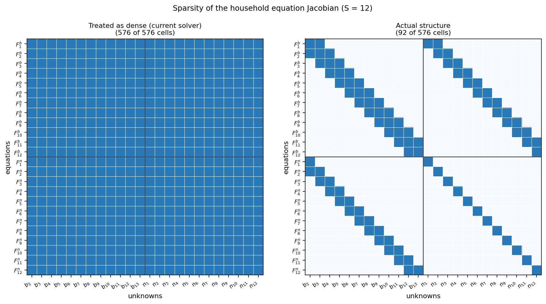
Fig. 4 Sparsity pattern of the household equation Jacobian, at \(S = 12\). Left: the standard finite-difference solve treats every entry of the \(2S\times 2S\) matrix as live (\((2S)^2 = 576\) entries). Right: the actual structure—each Euler equation depends only on a household’s own age and its immediate neighbors, leaving most entries zero (92 of 576 here; 636 of 25{,}600 at the default \(S = 80\)).#
The steady-state solution method for each of the cases above is associated with a solution method that has a subset of the following outer-loop variables \(\Bigl\{\bar{r}_p, \bar{r}, \bar{w}, \{\bar{p}_m\}_{m=1}^{M-1}, \bar{Y}, \overline{TR}, \overline{BQ}, factor\Bigr\}\).
Stationary Steady-State Equilibrium Definition#
With the stationarized model, we can now define the stationary steady-state equilibrium. This equilibrium will be long-run values of the endogenous variables that are constant over time. In a perfect foresight model, the steady-state equilibrium is the state of the economy at which the model settles after a finite amount of time, regardless of the initial condition of the model. Once the model arrives at the steady-state, it stays there indefinitely unless it receives some type of shock or stimulus.
These stationary values have all the components of growth, from productivity growth and population growth, removed as defined in Table 3. This is possible because the productivity growth rate \(g_y\) and population growth rate series \(\tilde{g}_{n,t}\) are exogenous. We can transform the stationary equilibrium values of the variables back to their nonstationary values by reversing the identities in Table 3.
We define a stationary steady-state equilibrium as the following.
Definition: Stationary steady-state equilibrium
A non-autarkic stationary steady-state equilibrium in the OG-Core model is defined as constant allocations of stationary household labor supply \(n_{j,s,t}=\bar{n}_{j,s}\) and savings \(\hat{b}_{j,s+1,t+1}=\bar{b}_{j,s+1}\) for all \(j\), \(t\), and \(E+1\leq s\leq E+S\), and constant prices \(\hat{w}_t=\bar{w}\), \(r_t=\bar{r}\), \(r_{p,t}=\bar{r}_p\), \(\{p_{m,t}\}_{m=1}^M = \{\bar{p}_m\}_{m=1}^M\), and \(p_t=\bar{p}\) for all \(t\) such that the following conditions hold:
The population has reached its stationary steady-state distribution \(\hat{\omega}_{s,t} = \bar{\omega}_s\) for all \(s\) and \(t\) as characterized in Section Population steady-state and transition path,
households optimize according to (128), (129), (130), and (125),
firms in each industry optimize according to (135) and (136),
government activity behaves according to (94), (145), (150), and (152), and
markets clear according to (161), (165), (166), (169), (170), and (173).
Steady-state solution method#
The default specification of the model is the baseline specification (baseline = True) in which the government can run deficits and surpluses (budget_balance = False), in which the economy is a large partially open economy [\(\zeta_D,\zeta_K\in(0,1)\)], and in which baseline government spending \(G\) and transfers \(TR\) are not held at baseline levels (baseline_spending = False). We describe the algorithm for this model configuration below and follow that with a description of how it is modified for alternative configurations.
The computational algorithm for solving for the steady-state follows the steps below.
Use the techniques from Section Population steady-state and transition path to solve for the steady-state population distribution vector \(\boldsymbol{\bar{\omega}}\) and steady-state growth rate \(\bar{g}_n\) of the exogenous population process.
Choose an initial guess for the values of the steady-state interest rate (the after-tax marginal product of capital) \(\bar{r}^i\), wage rate \(\bar{w}^i\), portfolio rate of return \(\bar{r}_p^i\), output prices \(\{\bar{p}_m^i\}_{m=1}^{M-1}\) (note that \(\bar{p}_M =1\) since it’s the numeraire good), total bequests \(\overline{BQ}^{\,i}\), total household transfers \(\overline{TR}^{\,i}\), and income multiplier \(factor^i\), where superscript \(i\) is the index of the iteration number of the guess \(\Bigl\{\bar{r}_p^i, \bar{r}^i, \bar{w}^i, \{\bar{p}_m^i\}_{m=1}^{M-1}, \overline{TR}^i, \overline{BQ}^i, factor^i\Bigr\}\).
Given \(\{\bar{p}_m^i\}_{m=1}^{M-1}\) find the price of consumption goods \(\{\bar{p}_i\}_{i=1}^I\) using (18)
From price of consumption goods, determine the price of the composite consmpution good, \(\bar{p}\) using equation (20)
Using (32) with \(\overline{TR}^{\,i}\), find transfers to each household, \(\overline{tr}_{j,s}\)
Use (142) to get aggregate GDP \(\overline{Y}\) from steady-state transfers \(\overline{TR}^i\).
With \(\overline{Y}\), use (131) to get \(\overline{RM}\) and use (132) to get \(\overline{rm}_{j,s}\).
Using the bequest transfer process, (27) and aggregate bequests, \(\overline{BQ}^{\,i}\), find \(bq_{j,s}\)
Given values \(\bar{p}^i\), \(\bar{r}_{p}^i\), \(\bar{w}^i\) \(\overline{bq}_{j,s}\), \(\overline{rm}_{j,s}\), \(\overline{tr}_{j,s}\), and \(factor^i\), solve for the steady-state household labor supply \(\bar{n}_{j,s}\) and savings \(\bar{b}_{j,s+1}\) decisions for all \(j\) and \(E+1\leq s\leq E+S\).
Each of the \(j\in 1,2,...J\) sets of \(2S\) steady-state Euler equations can be solved separately.
OG-Coreparallelizes this process using the maximum number of processors possible (up to \(J\) processors). Solve each system of Euler equations using a multivariate root-finder to solve the \(2S\) necessary conditions of the household given by the following steady-state versions of stationarized household Euler equations (128), (129), and (130) simultaneously for each \(j\), where steady-state composite consumption \(\bar{c}_{j,s}\) is given by the budget constraint (127).
(174)#\[\begin{split} \bar{c}_{j,s} &= \Bigl[(1 + \bar{r}_{p}^i)\bar{b}_{j,s} + \bar{w}^i e_{j,s}\bar{n}_{j,s} - \sum_{i=1}^I\left(1 + \tau_i^c\right)\bar{p}_i \bar{c}_{min,i} - e^{g_y}\bar{b}_{j,s+1} ... \\ &\qquad + \overline{bq}_{j,s} + \overline{rm}_{j,s} + \overline{tr}_{j,s} + \overline{ubi}_{j,s} + \overline{pension}_{j,s} - \overline{tax}_{j,s}\Bigr] / \bar{p} \\ &\qquad\qquad\forall j\quad\text{and}\quad E+1\leq s\leq E+S \quad\text{where}\quad \bar{b}_{j,E+1}=0\end{split}\](175)#\[\begin{split} \frac{\bar{w}^i e_{j,s}}{\bar{p}}\bigl(1 - \tau^{mtrx}_{s}\bigr)(\bar{c}_{j,s})^{-\sigma} = \chi^n_{s}\biggl(\frac{b}{\tilde{l}}\biggr)\biggl(\frac{\bar{n}_{j,s}}{\tilde{l}}\biggr)^{\upsilon-1}\Biggl[1 - \biggl(\frac{\bar{n}_{j,s}}{\tilde{l}}\biggr)^\upsilon\Biggr]^{\frac{1-\upsilon}{\upsilon}} \\ \qquad\qquad\qquad\qquad\qquad\qquad\qquad\qquad\forall j \quad\text{and}\quad E+1\leq s\leq E+S \\\end{split}\](176)#\[\begin{split} \frac{(\bar{c}_{j,s})^{-\sigma}}{\bar{p}} &= e^{-\sigma g_y}\Biggl[\chi^b_j\rho_s(\bar{b}_{j,s+1})^{-\sigma} ... \\ &\quad\quad\quad + \beta_j\bigl(1 - \rho_s\bigr)\left(\frac{1 + \bar{r}_{p}^i\bigl[1 - \tau^{mtry}_{s+1}\bigr] - \tau^{mtrw}}{\bar{p}}\right)(\bar{c}_{j,s+1})^{-\sigma}\Biggr] \\ &\qquad\qquad\qquad\qquad\qquad\qquad\forall j \quad\text{and}\quad E+1\leq s\leq E+S-1 \\\end{split}\](177)#\[ \frac{(\bar{c}_{j,E+S})^{-\sigma}}{\bar{p}} = e^{-\sigma g_y}\chi^b_j(\bar{b}_{j,E+S+1})^{-\sigma} \quad\forall j\]Determine from the quantity of the composite consumption good consumed by each household, \(\bar{c}_{j,s}\), use equation (125) to determine consumption of each output good, \(\bar{c}_{m,j,s}\)
Using \(\bar{c}_{m,j,s}\) in (119), solve for aggregate consumption of each output good, \(\bar{C}_{m}\)
Given values for \(\bar{n}_{j,s}\) and \(\bar{b}_{j,s+1}\) for all \(j\) and \(s\), solve for steady-state labor supply, \(\bar{L}\), savings, \(\bar{B}\)
Use \(\bar{n}_{j,s}\) and the steady-state version of the stationarized labor market clearing equation (161) to get a value for \(\bar{L}^{i}\).
(178)#\[ \bar{L} = \sum_{s=E+1}^{E+S}\sum_{j=1}^{J} \bar{\omega}_{s}\lambda_j e_{j,s}\bar{n}_{j,s}\]Use \(\bar{b}_{j,s+1}\) and the steady-state version of the stationarized expression for total savings by domestic households (162)to solve for \(\bar{B}\).
(179)#\[ \bar{B} \equiv \frac{1}{1 + \bar{g}_{n}}\sum_{s=E+2}^{E+S+1}\sum_{j=1}^{J}\Bigl(\bar{\omega}_{s-1}\lambda_j\bar{b}_{j,s} + i_s\bar{\omega}_{s}\lambda_j\bar{b}_{j,s}\Bigr)\]
Solve for the exogenous government interest rate \(\bar{r}_{gov}\) using equation (94).
Use (151) to find \(\overline{D}\) from \(\overline{Y}\)
Using \(\overline{D}\), we can find foreign investor holdings of debt, \(\overline{D}^{f}\) from (104) and then solve for domestic debt holdings through the debt market clearing condition: \(\overline{D}^{d} = \overline{D} - \overline{D}^{f}\)
Using \(\overline{Y}\), find government infrastructure investment, \(\bar{I}_{g}\) from (146)
Using the law of motion of the stock of infrastructure, (148), and \(\bar{I}_{g}\), solve for \(\overline{K}_{g}\)
Find output and factor demands for M-1 industries:
By (169), \(\overline{Y}_{m}=\overline{C}_{m}\) for \(1\leq m \leq M-1\), where \(\overline{C}_{m}\) is determined by (171).
The capital-output ratio can be determined from the FOC for the firms’ choice of capital: \(\frac{\bar{K}_m}{\bar{Y}_m} = \gamma_m\left[\frac{\bar{r} +\bar{\delta}_M - \bar{\tau}^{corp}_m\bar{\delta}^{\tau}_m - \bar{\tau}^{inv}_m\bar{\delta}_M}{\left(1 - \bar{\tau}^{corp}_m\right)\bar{p}_m(\bar{Z}_m)^\frac{\varepsilon_m-1}{\varepsilon_m}}\right]^{-\varepsilon_m}\)
Capital demand can thus be found: \(\bar{K}_{m} = \frac{\bar{K}_m}{\bar{Y}_m} * \bar{Y}_m\)
Labor demand can be found by inverting the production function:
(180)#\[ \bar{L}_{m} = \left(\frac{\left(\frac{\bar{Y}_m}{\bar{Z}_m}\right)^{\frac{\varepsilon_m-1}{\varepsilon_m}} - \gamma_{m}^{\frac{1}{\varepsilon_m}}\bar{K}_m^{\frac{\varepsilon_m-1}{\varepsilon_m}} - \gamma_{g,m}^{\frac{1}{\varepsilon_m}}\bar{K}_{g,m}^{\frac{\varepsilon_m-1}{\varepsilon_m}}}{(1-\gamma_m-\gamma_{g,m})^{\frac{1}{\varepsilon_m}}}\right)^{\frac{\varepsilon_m}{\varepsilon_m-1}}\]Use the steady-state world interest rate \(\bar{r}^*\) and labor demand \(\bar{L}_m\) to solve for private capital demand at the world interest rate \(\bar{K}_m^{r^*}\) using the steady-state version of (50)
(181)#\[ \bar{K}_m^{r^*} = \bar{L}_m\left(\frac{\bar{w}}{\frac{\bar{r} + \bar{\delta}_M - \bar{\tau}^{corp}_m\bar{\delta}^{\tau}_m - \bar{\tau}^{inv}_m\bar{\delta}_M}{1 - \bar{\tau}^{corp}_m}}\right)^{\varepsilon_m} \frac{\gamma_m}{(1 - \gamma_m - \gamma_{g,m})}\]
Determine factor demands and output for industry \(M\):
\(\bar{L}_M = \bar{L} - \sum_{m=1}^{M-1}\bar{L}_{m}\)
Find \(\bar{K}_m^{r^*}\) using the steady-state version of (50)
Find total capital supply, and the split between that from domestic and foreign households: \(\bar{K}\), \(\bar{K}^d\), \(\bar{K}^f\):
We then use this to find foreign demand for domestic capital from (107): \(\bar{K}^{f} = \bar{\zeta}_{K}\sum_{m=1}^{M}\bar{K}_m^{r^*}\)
Using \(\bar{D}^{d}\) we can then find domestic investors’ holdings of private capital as the residual from their total asset holdings: , \(\bar{K}^{d} = \bar{B} - \bar{D}^{d}\)
Aggregate capital supply is then determined as \(\bar{K} = \bar{K}^{d} + \bar{K}^{f}\).
\(\bar{K}_M = \bar{K} - \sum_{m=1}^{M-1}\bar{K}_{m}\)
Use the factor demands and \(\bar{K}_g\) in the production function for industry \(M\) to find \(\bar{Y}_M\).
Find an updated value for GDP, \(\bar{Y}^{i'} = \sum_{m=1}^{M} \bar{p}_m\bar{Y}_m\) using (141).
Find a updated values for \(\bar{I}_{g}^{i'}\) and \(\bar{K}_g^{i'}\) using \(\bar{Y}^{i'}\) and equations (146) and (148)
Given updated inner-loop values based on initial guesses for outer-loop variables \(\Bigl\{\bar{r}_p^i, \bar{r}^i, \bar{w}^i, \bigl\{\bar{p}_m^i\bigr\}_{m=1}^{M-1}, \overline{BQ}^i, \overline{TR}^i, factor^i\Bigr\}\), solve for updated values of outer-loop variables \(\Bigl\{\bar{r}_p^{i'}, \bar{r}^{i'}, \bar{w}^{i'}, \bigl\{\bar{p}_m^{i'}\bigr\}_{m=1}^{M-1}, \overline{BQ}^{i'}, \overline{TR}^{i'}, factor^{i'}\Bigr\}\) using the remaining equations:
Use \(\bar{Y}_M\) and \(\bar{K}_M\) in (136) to solve for updated value of the rental rate on private capital \(\bar{r}^{i'}\).
Use \(\bar{Y}_M\) and \(\bar{L}_M\) in (135) to solve for updated value of the wage rate \(\bar{w}^{i'}\).
Use \(\bar{r}^{i'}\) in equation (94) to get \(\bar{r}_{gov}^{i'}\)
Use \(\bar{K}_g^{i'}\) and \(\bar{Y}^{i'}\) in (50) for each industry \(m\) to solve for the value of the marginal product of government capital in each industry, \(\overline{MPK}_{g,m}\)
Use \(\boldsymbol{\overline{MPK}}_g\), \(\bar{r}^{i'}\), \(\bar{r}_{gov}^{i'}\), \(\bar{D}\), and \(\bar{K}\) to find the return on the households’ investment portfolio \(\bar{r}_{p}^{i'}\) using equation (150).
Use \(\bar{Y}_m\), \(\bar{L}_m\) in (135) to solve for the updates vector of prices, \(\{\bar{p}_m^{i'}\}_{m=1}^{M-1}\).
Use \(\bar{r}_{p}^{i'}\) and \(\bar{b}_{j,s}\) in (173) to solve for updated aggregate bequests \(\overline{BQ}^{i'}\).
Use \(\bar{Y}^{i'}\) in the long-run aggregate transfers assumption (142) to get an updated value for total transfers to households \(\overline{TR}^{i'}\). Note that this \(\bar{Y}^{i'}\) is different from the \(\bar{Y}\) derived from the initial guess of aggregate transfers \(\overline{TR}^i\) from step 2.4.
Use \(\bar{r}^{i'}\), \(\bar{r}_{p}^{i}\), \(\bar{w}^{i'}\), \(\bar{n}_{j,s}\), and \(\bar{b}_{j,s+1}\) in equation (182) to get an updated value for the income factor \(factor^{i'}\).
(182)#\[\begin{split} factor^{i'} &= \frac{\text{Avg. household income in data}}{\text{Avg. household income in model}} \\ &= \frac{\text{Avg. household income in data}}{\sum_{s=E+1}^{E+S}\sum_{j=1}^J \lambda_j\bar{\omega}_s\left(\bar{r}_{p}^{i'}\bar{b}_{j,s} + \bar{w}^{i'} e_{j,s}\bar{n}_{j,s}\right)} \quad\forall t\end{split}\]
If the updated values of the outer-loop variables \(\Bigl\{\bar{r}_p^{i'}, \bar{r}^{i'}, \bar{w}^{i'}, \{\bar{p}_m^{i'}\}_{m=1}^{M-1}, \overline{BQ}^{i'}, \overline{TR}^{i'}, factor^{i'}\Bigr\}\) are close enough to the initial guess for the outer-loop variables \(\Bigl\{\bar{r}_p^i, \bar{r}^i, \bar{w}^{i}, \{\bar{p}_m^{i}\}_{m=1}^{M-1}, \overline{BQ}^i, \overline{TR}^i, factor^i\Bigr\}\) then the fixed point is found and the steady-state equilibrium is the fixed point solution. If the outer-loop variables are not close enough to the initial guess for the outer-loop variables, then update the initial guess of the outer-loop variables \(\Bigl\{\bar{r}_p^{i+1}, \bar{r}^{i+1}, \bar{w}^{i+1}, \{\bar{p}_m^{i+1}\}_{m=1}^{M-1}, \overline{BQ}^{i+1}, \overline{TR}^{i+1}, factor^{i+1}\Bigr\}\) as a convex combination of the first initial guess \(\Bigl\{\bar{r}_p^{i}, \bar{r}^{i}, \bar{w}^{i}, \{\bar{p}_m^{i}\}_{m=1}^{M-1}, \overline{BQ}^{i}, \overline{TR}^{i}, factor^{i}\Bigr\}\) and the updated values \(\Bigl\{\bar{r}_p^{i'}, \bar{r}^{i'}, \bar{w}^{i'}, \{\bar{p}_m^{i'}\}_{m=1}^{M-1}, \overline{BQ}^{i'}, \overline{TR}^{i'}, factor^{i'}\Bigr\}\) and repeat steps (2) through (4).
Define a tolerance \(toler_{ss,out}\) and a distance metric \(\left\lVert\,\cdot\,\right\rVert\) on the space of 7-tuples of outer-loop variables \(\{\bar{r}_p^{i}, \bar{r}^{i}, \bar{w}^{i}, \{\bar{p}_m^{i}\}_{m=1}^{M-1}, \overline{BQ}^{i}, \overline{TR}^{i}, factor^{i}\}\). If the distance between the original guess for the outer-loop variables and the updated values for the outer-loop variables is less-than-or-equal-to the tolerance value, then the steady-state equilibrium has been found and it is the fixed point values of the variables at this point in the iteration.
(183)#\[\begin{split} & \Biggl\lVert\left(\bar{r}_p^{i'}, \bar{r}^{i'}, \bar{w}^{i'}, \{\bar{p}_m^{i'}\}_{m=1}^{M-1}, \overline{BQ}^{i'}, \overline{TR}^{i'}, factor^{i'}\right) ... \\ &\qquad - \left(\bar{r}_p^{i}, \bar{r}^{i}, \bar{w}^{i}, \{\bar{p}_m^{i}\}_{m=1}^{M-1}, \overline{BQ}^{i}, \overline{TR}^{i}, factor^{i}\right)\Biggr\rVert \leq toler_{ss,out}\end{split}\]Make sure that steady-state government spending is nonnegative \(\bar{G}\geq 0\). If steady-state government spending is negative, that means the government is getting resources to supply the debt from outside the economy each period to stabilize the debt-to-GDP ratio. \(\bar{G}<0\) is a good indicator of unsustainable policies.
Make sure that the resource constraint (goods market clearing) (170) is satisfied. It is redundant, but this is a good check as to whether everything worked correctly.
Make sure that the government budget constraint (145) binds.
Make sure that all the \(2JS\) household Euler equations are solved to a satisfactory tolerance.
If the distance metric of the original value of the outer-loop variables and the updated values is greater than the tolerance \(toler_{ss,out}\), then an updated initial guess for the outer-loop variables is made as a convex combination of the first guess and the updated guess and steps (2) through (4) are repeated.
The distance metric not being satisfied is the following condition.
(184)#\[\begin{split} &\Biggl\lVert\left(\bar{r}_p^{i'}, \bar{r}^{i'}, \bar{w}^{i'}, \{\bar{p}_m^{i'}\}_{m=1}^{M-1}, \overline{BQ}^{i'}, \overline{TR}^{i'}, factor^{i'}\right) ... \\ &\qquad - \left(\bar{r}_p^{i}, \bar{r}^{i}, \bar{w}^{i}, \{\bar{p}_m^{i}\}_{m=1}^{M-1}, \overline{BQ}^{i}, \overline{TR}^{i}, factor^{i}\right)\Biggr\rVert > toler_{ss,out}\end{split}\]If the distance metric is not satisfied (184), then an updated initial guess for the outer-loop variables \(\Bigl\{\bar{r}_p^{i+1}, \bar{r}^{i+1}, \bar{w}^{i+1}, \{\bar{p}_m^{i+1}\}_{m=1}^{M-1}, \overline{BQ}^{i+1}, \overline{TR}^{i+1}, factor^{i+1}\Bigr\}\) is made as a convex combination of the previous initial guess \(\Bigl\{\bar{r}_p^{i}, \bar{r}^{i}, \bar{w}^{i}, \{\bar{p}_m^{i}\}_{m=1}^{M-1}, \overline{BQ}^{i}, \overline{TR}^{i}, factor^{i}\Bigr\}\) and the updated values based on the previous initial guess \(\Bigl\{\bar{r}_p^{i'}, \bar{r}^{i'}, \bar{w}^{i'}, \{\bar{p}_m^{i'}\}_{m=1}^{M-1}, \overline{BQ}^{i'}, \overline{TR}^{i'}, factor^{i'}\Bigr\}\) and repeats steps (2) through (4) with this new initial guess. The parameter \(\xi_{ss}\in(0,1]\) governs the degree to which the new guess \(i+1\) is close to the updated guess \(i'\).
(185)#\[\begin{split} & \left(\bar{r}_p^{i+1}, \bar{r}^{i+1}, \bar{w}^{i+1}, \{\bar{p}_m^{i+1}\}_{m=1}^{M-1}, \overline{BQ}^{i+1}, \overline{TR}^{i+1}, factor^{i+1}\right) = ... \\ &\qquad \xi_{ss}\left(\bar{r}_p^{i'}, \bar{r}^{i'}, \bar{w}^{i'}, \{\bar{p}_m^{i'}\}_{m=1}^{M-1}, \overline{BQ}^{i'}, \overline{TR}^{i'}, factor^{i'}\right) + ... \\ &\qquad(1-\xi_{ss})\left(\bar{r}_p^{i}, \bar{r}^{i}, \bar{w}^{i}, \{\bar{p}_m^{i}\}_{m=1}^{M-1}, \overline{BQ}^{i}, \overline{TR}^{i}, factor^{i}\right)\end{split}\]Because the outer loop of the steady-state solution has \(M-1+6\) variables, there are \(M+5\) functions to minimize or set to zero. We use a root-finder and its corresponding Newton method for the updating the guesses of the outer-loop variables because it works well and is faster than the bisection method described in the previous step. The
OG-Corecode has the option to use either the bisection method or the root fining method to updated the outer-loop variables. The root finding algorithm is generally faster but is less robust than the bisection method in the previous step.
Under alternative model configurations, the solution algorithm changes slightly. For example, when baseline = False, one need not solve for the \(factor\), as it is determined in the baseline model solution. When budget_balance = True, the guess of \(\overline{TR}\) in the outer loop is replaced by the guess of \(\bar{Y}\) and transfers are determined a residual from the government budget constraint given revenues and other spending policy. When baseline_spending = True, \(\overline{TR}\) is determined from the baseline model solution and not updated in the outer loop described above. In this case, \(\bar{Y}\) becomes an outer loop variable.
Steady-state results: default specification#
[TODO: Update the results in this section.] In this section, we use the baseline calibration described in Chapter Calibrating OG-Core, which includes the baseline tax law from Tax-Calculator, to show some steady-state results from OG-Core. Figures Fig. 5, Fig. 6, and Fig. 7 show the household steady-state variables by age \(s\) and lifetime income group \(j\).
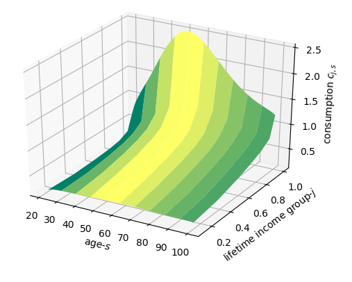
Fig. 5 Consumption \(c_{j,s}\) by age \(s\) and lifetime income group \(j\)#
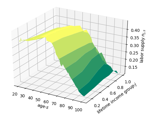
Fig. 6 Labor supply \(n_{j,s}\) by age \(s\) and lifetime income group \(j\)#
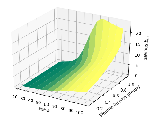
Fig. 7 Savings \(b_{j,s}\) by age \(s\) and lifetime income group \(j\)#
Table 4 lists the steady-state prices and aggregate variable values along with some of the maximum error values from the characterizing equations.
Variable |
Value |
Variable |
Value |
|---|---|---|---|
\(\bar{r}\) |
0.630 |
\(\bar{w}\) |
1.148 |
\(\bar{Y}\) |
0.630 |
\(\bar{C}\) |
0.462 |
\(\bar{I}\) |
0.144 |
\(\bar{K}\) |
1.810 |
\(\bar{L}\) |
0.357 |
\(\bar{B}\) |
2.440 |
\(\overline{BQ}\) |
0.106 |
\(factor\) |
141,580 |
\(\overline{Rev}\) |
0.096 |
\(\overline{TR}\) |
0.057 |
\(\bar{G}\) |
0.023 |
\(\bar{D}\) |
0.630 |
Max. abs. labor supply Euler error |
4.57e-13 |
Max. abs. savings Euler error |
8.52e-13 |
Resource constraint error |
-4.39e-15 |
Serial computation time |
1 hr. 25.9 sec. |
The steady-state computation time does not include any of the exogenous parameter computation processes, the longest of which is the estimation of the baseline tax functions which computation takes 1 hour and 15 minutes.
Stationary Non-Steady-State Equilibrium#
In this section, we define the stationary non-steady-state equilibrium of the OG-Core model. Chapters Households through Market Clearing derive the equations that characterize the equilibrium of the model in their non-stationarized form. And chapter Stationarization derives the stationarized versions of the characterizing equations. The steady-state equilibrium definition in Section Stationary Steady-State Equilibrium Definition defines the long-run equilibrium where the economy settles down after many periods. The non-steady-state equilibrium in this section describes the equilibrium in all periods from the current period to the steady-state. We will need the steady-state solution from Section Stationary Steady-State Equilibirum to solve for the non-steady-state equilibrium transition path.
Stationary Non-Steady-State Equilibrium Definition#
We define a stationary non-steady-state equilibrium as the following.
Definition: Stationary Non-steady-state functional equilibrium
A non-autarkic non-steady-state functional equilibrium in the OG-Core model is defined as stationary allocation functions of the state \(\bigl\{n_{j,s,t} = \phi_{j,s}\bigl(\boldsymbol{\hat{\Gamma}}_t\bigr)\bigr\}_{s=E+1}^{E+S}\) and \(\bigl\{\hat{b}_{j,s+1,t+1}=\psi_{j,s}\bigl(\boldsymbol{\hat{\Gamma}}_t\bigr)\bigr\}_{s=E+1}^{E+S}\) for all \(j\) and \(t\) and stationary price functions \(\hat{w}(\boldsymbol{\hat{\Gamma}}_t)\), \(r(\boldsymbol{\hat{\Gamma}}_t)\), and \(\boldsymbol{p}(\boldsymbol{\hat{\Gamma}}_t)\) for all \(t\) such that:
Households have symmetric beliefs \(\Omega(\cdot)\) about the evolution of the distribution of savings as characterized in (41), and those beliefs about the future distribution of savings equal the realized outcome (rational expectations),
Stationary non-steady-state solution method#
This section describes the computational algorithm for the solution method for the stationary non-steady-state equilibrium described in the Stationary Non-Steady-State Equilibrium Definition. The default specification of the model is the baseline specification (baseline = True) in which the government can run deficits and surpluses (budget_balance = False), in which the economy is a large partially open economy [\(\zeta_D,\zeta_K\in(0,1)\)], and in which baseline government spending \(G_t\) and transfers \(TR_t\) are not held constant until the closure rule (baseline_spending = False). We describe the algorithm for this model configuration below and follow that with a description of how it is modified for alternative configurations.
The computational algorithm for the non-steady-state solution follows similar steps to the steady-state solution described in Section Steady-state solution method. There is an outer-loop of guessed time series values of macroeconomic variables \(\Bigl\{r_{p,t}, r_t, w_t, \{p_{m,t}\}_{m=1}^{M-1}, BQ_t, TR_t\Bigr\}_{t=1}^T\). Note that in the case of the transition path equilibrium algorithm, we guess the time series of those variables from the current period \(t=1\) to the steady state (\(t=T\)). Then we solve the inner loop of mostly microeconomic variables for the whole transition path (many generations of households), given the outer-loop guesses. We iterate between these steps until we find a fixed point.
We call this solution algorithm the time path iteration (TPI) method or transition path iteration. This method was originally outlined in a series of papers between 1981 and 1985 [1] and in the seminal book [Auerbach and Kotlikoff, 1987] [Chapter 4] for the perfect foresight case and in [Nishiyama and Smetters, 2007] Appendix II and [Evans and Phillips, 2014][Sec. 3.1] for the stochastic case. The intuition for the TPI solution method is that the economy is infinitely lived, even though the agents that make up the economy are not. Rather than recursively solving for equilibrium policy functions by iterating on individual value functions, one must recursively solve for the policy functions by iterating on the entire transition path of the endogenous objects in the economy (see [Stokey et al., 1989] [Chapter 17]).
The key assumption is that the economy will reach the steady-state equilibrium \(\boldsymbol{\bar{\Gamma}}\) described in Stationary Steady-State Equilibrium Definition in a finite number of periods \(T<\infty\) regardless of the initial state \(\boldsymbol{\hat{\Gamma}}_1\). The first step in solving for the non-steady-state equilibrium transition path is to solve for the steady-state using the method described in Section Steady-state solution method. After solving for the steady-state, one must then find a fixed point over the entire time path or transition path of endogenous objects that satisfies the characterizing equilibrium equations in every period.
The stationary non-steady state (transition path) solution algorithm has following steps.
Use the techniques from Section Population steady-state and transition path to solve for the transition path of the stationarized population distribution matrix \(\{\hat{\omega}_{s,t}\}_{s,t=E+1,1}^{E+S,T}\) and population growth rate vector \(\{\tilde{g}_{n,t}\}_{t=1}^T\) of the exogenous population process.
Compute the steady-state solution \(\{\bar{n}_{j,s},\bar{b}_{j,s+1}\}_{s=E+1}^{E+S}\) corresponding to Stationary Steady-State Equilibrium Definition with the Steady-state solution method.
Given initial state of the economy \(\boldsymbol{\hat{\Gamma}}_1\) and steady-state solutions \(\{\bar{n}_{j,s},\bar{b}_{j,s+1}\}_{s=E+1}^{E+S}\), guess transition paths of outer-loop macroeconomic variables \(\Bigl\{\boldsymbol{r}_p^i, \boldsymbol{r}^i, \boldsymbol{\hat{w}}^i, \{\boldsymbol{p}_m^i\}_{m=1}^{M-1}, \boldsymbol{\hat{BQ}}^i,\boldsymbol{\hat{TR}}^i\Bigr\}\) such that \(\hat{BQ}_1^i\) is consistent with \(\boldsymbol{\hat{\Gamma}}_1\) and \(\Bigl\{r_{p,t}^i, r_t^i, \hat{w}_t^i, \{p_{m,t}^i\}_{m=1}^{M-1}, \hat{BQ}_t^i, \hat{TR}_t^i\Bigr\} = \{\bar{r}_p, \bar{r}, \bar{w}, \{\bar{p}_m\}_{m=1}^{M-1}, \overline{BQ}, \overline{TR}\}\) for all \(t\geq T\). We also make an initial guess regarding the amount of government debt in each period, \(\boldsymbol{\hat{D}}^i\). This will not enter the ``outer loop’’ variables, but is helpful in the first pass through the time path iteration algorithm.
If the economy is assumed to reach the steady state by period \(T\), then we must be able to solve for every cohort’s decisions in period \(T\) including the decisions of agents in their first period of economically relevant life \(s=E+S\). This means we need to guess time paths for the outer-loop variables that extend to period \(t=T+S\). However, the values of the time path of outer-loop variables for every period \(t\geq T\) are simply equal to the steady-state values.
Using (32) with \(\boldsymbol{\hat{TR}}^{\,i}\), find transfers to each household \(\hat{tr}_{j,s,t}\).
Using the bequest transfer process, (27) and aggregate bequests, \(\boldsymbol{\hat{BQ}}^{\,i}\), find bequests received by each household \(\hat{bq}_{j,s,t}\).
Given time path guesses for \(\boldsymbol{r}_p^i\), \(\boldsymbol{\hat{w}}^i\), and \(\{\boldsymbol{p}_m^i\}_{m=1}^{M-1}\), and the transition paths of household received bequests \(\hat{bq}_{j,s,t}\) and government transfers to households \(\hat{tr}_{j,s,t}\), we can solve for each household’s lifetime decisions \(\{n_{j,s,t},\hat{b}_{j,s+1,t+1}\}_{s=E+1}^{E+S}\) for all \(j\), \(E+1\leq s \leq E+S\), and \(1\leq t\leq T+S-1\).
Given the prices of production goods \(\{\boldsymbol{p}_m^i\}_{m=1}^{M-1}\), find the transition path of the price of consumption goods \(p_{i,t}\) using (18).
From price of consumption goods \(p_{i,t}\), determine the price of the composite consmpution good, \(p_t\) using equation (20)
The household problem can be solved with a multivariate root finder solving the \(2S\) equations and unknowns at once for each \(j\) and \(1\leq t\leq T+S-1\). The root finder uses \(2S\) household Euler equations (128), (129), and (130) to solve for each household’s \(2S\) lifetime decisions. The household decision rules for each type and birth cohort are solved separately.
After solving the first iteration of time path iteration, subsequent initial values for the \(J\), \(2S\) root finding problems are based on the solution in the prior iteration. This speeds up computation further and makes the initial guess for the highly nonlinear system of equations start closer to the solution value.
Use the quantity of the composite consumption good consumed by each household, \(\hat{c}_{j,s,t}\) and equation (125) to determine consumption of each output good, \(\hat{c}_{m,j,s,t}\).
Using \(\hat{c}_{m,j,s,t}\) in (119), solve for aggregate consumption of each output good, \(\hat{C}_{m,t}\)
Given values for \(n_{j,s,t}\) and \(\hat{b}_{j,s+1,t+1}\) for all \(j\), \(s\), and \(t\), solve for aggregate labor supply, \(\hat{L}_t\), and savings, \(B_t\) in each period
Solve for the exogenous government interest rate \(r_{gov,t}^{i}\) using equation (94).
Use (142) to find \(\hat{Y}_t^i\) from the guess of \(\hat{TR}_t^i\)
Using the path of output from each industry, \(\hat{Y}_{m,t}\), and the household savings and labor supply decisions, \(\{n_{j,s,t},\hat{b}_{j,s+1,t+1}\}_{s=E+1}^{E+S}\), compute the path of stationarizaed total tax revenue, \(\hat{Revenue}_{t}^{i}\).
Using the long-run debt-to-GDP ratio, the path of GDP, \(\hat{Y}_t^i\), the path of total tax revenue, \(\hat{Revenue}_{t}^{i}\), government transfers, \(\hat{TR}_t^i\), infrastructure investment, \(\hat{I}_{g,t}^i\), and Equation (96), find the path of stationarized government debt, \(\hat{D}_{t}^{i'}\) for all \(t\).
Using \(\hat{D}_t^i\), we can find foreign investor holdings of debt, \(\hat{D}_t^{f,i}\) from (104) and then solve for domestic debt holdings through the debt market clearing condition: \(\hat{D}_t^{d,i} = \bar{D}_t^i - \bar{D}_t^{f,i}\)
Using \(\hat{Y}_t^i\), find government infrastructure investment, \(\hat{I}_{g,t}\) from (146)
Using the law of motion of the stock of infrastructure, (148), and \(\hat{I}_{g,t}\), solve for \(\hat{K}_{g,t}^{i}\)
Find output and factor demands for M-1 industries:
By (120), \(\hat{Y}_{m,t}=\hat{C}_{m,t}\), where \(\hat{C}_{m,t}\) is determined by (171)
The capital-output ratio can be determined from the FOC for the firms’ choice of capital: \(\frac{\hat{K}_{m,t}}{\hat{Y}_{m,t}} = \gamma_m\left[\frac{r_t + \delta_{M,t} - \tau^{corp}_{m,t}\delta^{\tau}_{m,t} - \tau^{inv}_{m,t}\delta_{M,t}}{(1-\tau^{corp}_{m,t})p_{m,t}({Z}_{m,t})^\frac{\varepsilon_m -1}{\varepsilon_m}}\right]^{-\varepsilon_m}\)
Capital demand can thus be found: \(\hat{K}_{m,t} = \frac{\hat{K}_{m,t}}{\hat{Y}_{m,t}} * \hat{Y}_{m,t}\)
Labor demand can be found by inverting the production function:
(186)#\[ \hat{L}_{m,t} = \left(\frac{\left(\frac{\hat{Y}_{m,t}}{Z_{m,t}}\right)^{\frac{\varepsilon_m-1}{\varepsilon_m}} - \gamma_{m}^{\frac{1}{\varepsilon_m}}\hat{K}_{m,t}^{\frac{\varepsilon_m-1}{\varepsilon_m}} - \gamma_{g,m}^{\frac{1}{\varepsilon_m}}\hat{K}_{g,m,t}^{\frac{\varepsilon_m-1}{\varepsilon_m}}}{(1-\gamma_m-\gamma_{g,m})^{\frac{1}{\varepsilon_m}}}\right)^{\frac{\varepsilon_m}{\varepsilon_m-1}}\]Use the interest rate \(r_t^*\) and labor demand \(\hat{L}_{m,t}\) to solve for private capital demand at the world interest rate \(\hat{K}_{m,t}^{r^*}\) using (50)
(187)#\[ \hat{K}_{m,t}^{r^*} = \hat{L}_{m,t}\left(\frac{\hat{w}_t}{\frac{r_t + \delta_{M,t} - \tau^{corp}_{m,t}\delta^{\tau}_{m,t} - \tau^{inv}_{m,t}\delta_{M,t}}{1 - \bar{\tau}_{m,t}^b}}\right)^{\varepsilon_m} \frac{\gamma_m}{(1 - \gamma_m - \gamma_{g,m})}\]Determine factor demands and output for industry \(M\):
\(\hat{L}_{M,t} = \hat{L}_t - \sum_{m=1}^{M-1}\hat{L}_{m,t}\)
Find \(\hat{K}_{m,t}^{r^*}\) using (50)
Find total capital supply, and the split between that from domestic and foreign households: \(\hat{K}_t^{i'}\), \(\hat{K}_t^d\), \(\hat{K}_t^f\):
We then use this to find foreign demand for domestic capital from (107): \(\hat{K}_t^{f} = \zeta_{K,t}\sum_{m=1}^{M}\hat{K}_{m,t}^{r^*}\)
Using \(\hat{D}_t^{d,i}\) we can then find domestic investors’ holdings of private capital as the residual from their total asset holdings: , \(\hat{K}_t^{d,i} = \hat{B}_t^i - \hat{D}_t^{d,i}\)
Aggregate capital supply is then determined as \(\hat{K}_t^{i'} = \hat{K}_t^{d,i} + \hat{K}_t^{f,i}\).
\(\hat{K}_{M,t} = \hat{K}_t^{i'} - \sum_{m=1}^{M-1}\hat{K}_{m,t}\)
Use the factor demands and \(\hat{K}_{g,t}\) in the production function for industry \(M\) to find \(\hat{Y}_{M,t}\)
Find an updated path for GDP, \(\hat{Y}_t^{i'} = \sum_{m=1}^{M} p_{m,t} \hat{Y}_{m,t}\)
Find a updated path for \(\hat{I}_{g,t}\) and \(\hat{K}_{g,t}\) using \(\hat{Y}_t^{i'}\), equations (146) and (148)
Given updated inner-loop values based on initial guesses for outer-loop variables \(\{r_{p,t}^i, r_t^i, \hat{w}_t^i, \boldsymbol{p}_t, \hat{BQ}_t^i, \hat{TR}_t^i\}\), solve for updated values of outer-loop variables \(\{r_{p,t}^{i'}, r_t^{i'}, \hat{w}_t^{i'}, \boldsymbol{p}_t^{i'}, \hat{BQ}_t^{i'}, \hat{TR}_t^{i'}\}\) using the remaining equations (for all periods \(t\) in the transition path):
Use \(\hat{Y}_{M,t}^{i'}\) and \(\hat{K}_{M,t}^{i'}\) in (136) to solve for updated value of the rental rate on private capital \(r_t^{i'}\).
Use \(\hat{Y}_{M,t}^{i'}\) and \(\hat{L}_{M,t}^{i}\) in (135) to solve for updated value of the wage rate \(\hat{w}_t^{i'}\).
Use \(r_t^{i'}\) in equations (94) to get \(r_{gov,t}^{i'}\)
Use \(\hat{K}_{g,t}^{i'}\) and \(\hat{Y}_t^{i''}\) in in (50) for each industry \(m\) to solve for the value of the marginal product of government capital in each industry, \(MPK_{g,m,t}^{i'}\)
Use \(\boldsymbol{MPK}_{g,t}^{i'}\), \(r_t^{i'}\), \(r_{gov,t}^{i'}\), \(\hat{D}_t^{i'}\), and \(\hat{K}_t^{i'}\) to find the return on the households’ investment portfolio, \(r_{p,t}^{i'}\)
Use \(\hat{Y}_{m,t}\), \(\hat{L}_{m,t}\) in (135) to solve for the updates vector of prices, \(\boldsymbol{p}_t^{i'}\)
Use \(r_{p,t}^{i'}\) and \(\hat{b}_{j,s,t}\) in (173) to solve for updated aggregate bequests \(\hat{BQ}_t^{i'}\).
Use \(\hat{Y}_t^{i'}\) in the aggregate transfers assumption (142) to get an updated value for total transfers to households \(\hat{TR}_t^{i'}\).
The updated values for the outer loop variables are then used to compute the percentage differences between the initial and implied values:
\(error_{r_p} = max\left\{\frac{r_{p,t}^{i'} - r_{p,t}^i}{r_{p,t}^i}\right\}_{t=0}^{T}\)
\(error_r = max\left\{\frac{r_{t}^{i'} - r_{t}^i}{r_{t}^i}\right\}_{t=0}^{T}\)
\(error_w = max\left\{\frac{\hat{w}_{t}^{i'} - \hat{w}_{t}^i}{\hat{w}_{t}^i}\right\}_{t=0}^{T}\)
\(error_p = max\left\{\frac{\boldsymbol{p}_{t}^{i'} - \boldsymbol{p}_{t}^i}{\boldsymbol{p}_{t}^i}\right\}_{t=0}^{T}\)
\(error_{bq} = max\left\{\frac{\hat{BQ}_{t}^{\,i'} - \hat{BQ}_{t}^{\,i}}{\hat{BQ}_{t}^{\,i}}\right\}_{t=0}^{T}\)
\(error_{tr} = \left\{\frac{\hat{TR}_{t}^{\,i'} - \hat{TR}_{t}^{\,i}}{\hat{TR}_{t}^{\,i}}\right\}_{t=0}^{T}\)
If the maximum absolute error among the four outer loop error terms is greater than some small positive tolerance \(toler_{tpi,out}\), \(\max\big|\left(error_{r_p}, error_r, error_w, error_p, error_{bq},error_{tr}\right)\bigr| > toler_{tpi,out}\), then update the guesses for the outer loop variables as a convex combination governed by \(\xi_{tpi}\in(0,1]\) of the respective initial guesses and the new implied values and repeat steps (3) through (23).
If the maximum absolute error among the M-1+5 outer loop error terms is less-than-or-equal-to some small positive tolerance \(toler_{tpi,out}\) in each period along the transition path, \(\max\big|\left(error_{r_p}, error_r, error_w, error_p, error_{bq},error_{tr}\right)\bigr| \leq toler_{tpi,out}\) then the non-steady-state equilibrium has been found.
Make sure that the resource constraint for industry \(M\) (goods market clearing) (170) is satisfied in each period along the time path. It is redundant, but this is a good check as to whether everything worked correctly.
Make sure that the government budget constraint (145) binds in every period.
Make sure that all the \((T+S)\times2JS\) household Euler equations are solved to a satisfactory tolerance in every period.
Under alternative model configurations, the solution algorithm changes slightly. When budget_balance = True, the guess of \(\boldsymbol{\hat{TR}}\) in the outer loop is replaced by the guess of \(\boldsymbol{\hat{Y}}\) and transfers are determined a residual from the government budget constraint given revenues and other spending policy. When baseline_spending = True, \(\boldsymbol{\hat{TR}}\) is determined from the baseline model solution and not updated in the outer loop described above. In this case \(\boldsymbol{\hat{Y}}\) becomes variable that is updates in the outer loop.
Baseline Non-steady-state Results#
[TODO: Add baseline non-steady-state results here.]
Footnotes#
This section contains the footnotes for this chapter.